-
[Machine Learning] 멀티 클래스 선형 분류(Multi-Class Linear Classification)Informatik 2022. 2. 22. 18:28
※ [Machine Learning] 베이즈 결정 이론(Bayesian Decision Theory)
[Machine Learning] 베이즈 결정 이론(Bayesian Decision Theory)
지도 학습(Supervised Learning)의 분류(Classification)에 해당하는 머신러닝(Machine Learning) 기법인 베이즈 결정 이론은 일상생활에서 흔하게 볼 수 있고 사용할 수 있는 기법이다. 예를 들어, 스팸 메일을.
minicokr.com
※ [Machine Learning] 선형 분류(Linear Classification)
[Machine Learning] 선형 분류(Linear Classification)
선형 분류는 일차원 혹은 다차원 데이터들을 선형 모델(Linear Model)을 이용하여 클래스들로 분류(Classification)하는 머신러닝(Machine Learning) 기법이다. 아래 예시는 2차원 데이터를 어떤 선형 모델로
minicokr.com
베이즈 결정 이론과 선형 분류 포스팅에서 이진 분류를 배웠고, 이번 포스팅에서는 멀티 클래스의 선형 분류를 다룬다.
3개 이상의 멀티 클래스 분류에서는 크게 세 가지 범주로 나눌 수 있다.
- 클래스 1개 vs. 전체 클래스
- 클래스 1개 vs. 클래스 1개
- 소프트맥스 회귀(Softmax Regression)
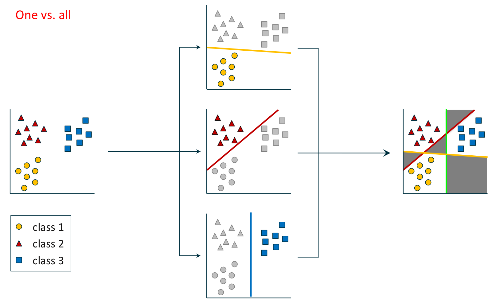
클래스 1개 vs. 전체 클래스
조건
- 클래스 레이블(Class Label) $\mathbf{Y} = \{1, \cdot, c\}$
- 학습 예제(Training Example) $(\mathbf {x}_1, y_1), \cdots, (\mathbf {x}_m, y_m)$
절차
- 각 클래스 레이블 $k \in \mathbf {Y}$에 대하여
- 학습 예제 $(\mathbf {x}_i, z_i)$를 다시 레이블링한다. where $$z_i = \begin {cases} 1 & : & y_i = k \\ 0 & : & \text{otherwise} \end {cases}$$
- 판별식 $h_k: \mathbb {R}^n \rightarrow \mathbb{R}$을 학습한다.
- $h_k(x)$가 가장 최대화되는 클래스 $k$로 분류한다.$$y = arg\max_{k \in \mathcal {Y}} h_k(\mathbf {x})$$
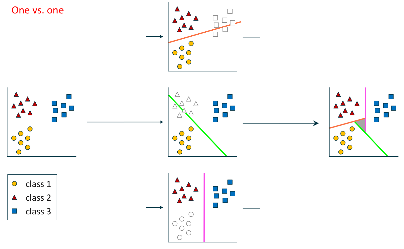
클래스 1개 vs. 전체 클래스
조건
- 클래스 레이블(Class Label) $\mathbf{Y} = \{1, \cdot, c\}$
- 학습 예제(Training Example) $(\mathbf {x}_1, y_1), \cdots, (\mathbf {x}_m, y_m)$
절차
- 각 클래스 레이블 $k, k' \in \mathbf {Y}$에 대하여 ($k < k'$)
- $D_{kk'} = D_k \cup D_{k'}$를 구성한다.
- 학습 예제 $(\mathbf {x}_i, z_i) \in D_{kk'}$를 다시 레이블링한다. where $$z_i = \begin {cases} 1 & : & y_i = k \\ 0 & : & y_i = k' \end {cases}$$
- 판별식 $h_{kk'}: \mathbb {R}^n \rightarrow \mathbb{R} \text{ using } D_{kk'}$을 학습한다.
- 다음과 같이 클래스 $k$로 분류한다. $$y = arg \max_{k \in \mathcal {Y}} \sum_{k' \in \mathcal {Y}} h_{kk'}(\mathbf {x})$$
※ [클래스 1개 vs. 전체 클래스] 방법에 비해 적은 수의 판별식인 $\frac{c(c - 1)}{2}$개를 갖는다.
소프트맥스 회귀(Softmax Regression)
가설(Hypothesis)
$$h_k(\mathbf {x}) = P(y = k | \mathbf {x}) = \frac {\exp (\mathbf {w}_k^{\top} \mathbf {x})}{\sum^c_{l = 1} \exp (\mathbf {w}_l^{\top} \mathbf {x})}, \ \ k = 1, \cdots, c$$
※ 카테고리 분포로 유도가 가능하다.
카테고리 분포(Categorical Distribution):
확률변수 $y$가 $\{1, \cdots c \}$ 중 하나의 값을 가질 때, 확률 함수는
$$P(y = k) = p_k, \text{ such that } \sum^c_{k = 1} p_k = 1$$이다. 다음과 같이 다른 표현 방법도 있다.
$$P(y) = \prod^c_{l = 1} p_l^{\mathbb {I} \{ y = l \}},\ \mathbb {I} \{ k = l \} = \begin {cases} 1, & k = l \\ 0, & k \neq l \end {cases}$$손실 함수(Loss Function)
$$J(\mathbf {w}_1, \cdots, \mathbf {w}_c) = - \frac {1}{m} \sum^m_{i = 1} \sum^c_{k = 1} \mathbb {I} \{ y_i = k \} \log h_k(\mathbf {x}_i)$$
경사(Gradient) = 손실 함수의 미분
$$\nabla_{\mathbf {w}_k} J(\mathbf {w}_1, \cdots, \mathbf {w}_c) = - \frac {1}{m} \sum^m_{i = 1} \left ( \mathbb {I} \{ y_i = k\} - h_l (\mathbf {x}_i) \right ) \mathbf {x}_i$$
소프트맥스 함수에서 각 가중치(Weight) $\mathbf {w}_k$에서 벡터 $\mathbf {v}$만큼 이동하더라도 결과에 영향이 없다.
$$h_k (\mathbf{x}; \mathbf{v}) = \frac {\exp ((\mathbf{w}_k - \mathbf{v})^{\top} \mathbf {x})}{\sum^c_{l = 1} \exp ((\mathbf {w}_l - \mathbf {v})^{\top} \mathbf {x})} = \frac {\exp (\mathbf {w}_k^{\top} \mathbf {x})}{\sum^c_{l = 1} \exp (\mathbf {w}_l^{\top} \mathbf {x})} = h_k (\mathbf {x})$$
$\mathbf {v} = \mathbf {w}_c$로 설정한다면, $h_1, \cdots, h_{c - 1}$를 결정하면서 $h_c$은 자동으로 결정이 된다. 특히, $c = 2$일 때, $h_1(\mathbf {x} ; \mathbf {w}_2) = \sigma((\mathbf {w}_1 - \mathbf {w}_2)^{\top} \mathbf {x})$ 로지스틱 회귀(Logistic Regression)의 식과 같다.
목표
미지수 함수를 추정하여라.
$$f: \mathcal {X} \rightarrow [0, 1]^c \ \ \ \ x \mapsto f(x) = (p_1(x), p_2(x), \cdots, p_c(x))^{\top}$$
such that $\sum^c_{k = 1} p_(x) = 1$ for all $x$
피벗 클래스(Pivot Class) $y = c$를 선택한다. 각 클래스 $k$와 피벗 클래스 $c$에 해당하는 두 로지스틱 회귀 모델을 하나의 식 $g'_k(\mathbf{x})$로 치환한다.
$$g'_k(\mathbf {x}) = p_k(\mathbf {x}) - p_c(\mathbf {x}), \ \ k = 1, \cdots, c - 1$$
각 로지스틱 회귀 모델의 판별식은 다음과 같다.
$$y = \begin {cases} k, & g'_k(\mathbf {x}) \geq 0 \\ c, & g'_k(\mathbf {x}) < 0 \end {cases}$$
같은 식을 다르게 표현하면 다음과 같다.
$$y = \begin {cases} k, & g'_k(\mathbf {x}) \geq 0 \\ c, & g'_k(\mathbf {x}) < 0 \end {cases},
\ \ \text {where } g_k (\mathbf {x}) = \log \frac {p_k(\mathbf {x})}{p_c(\mathbf {x})}, \ \ k = 1, \cdots, c - 1$$해당 판별식이 선형적이라고 가정하면,
$$g_k (\mathbf {x}) = \log \frac {p_k(\mathbf {x})}{p_c(\mathbf {x})} = \mathbf {w}^{\top}_k \mathbf {x}, \ \ k = 1, \cdots, c - 1$$
다음과 같은 로직스틱 회귀 모델에 도달할 수 있다.
$$\begin {align*}
p_k (\mathbf {x}) &= \frac {\exp (\mathbf {w}^{\top}_k \mathbf {x})}{1 + \sum^{c - 1}_{l = 1} \exp (\mathbf {w}^{\top}_l \mathbf {x})} & k = 1, \cdots, c - 1, \\
p_c(\mathbf {x}) &= \frac {1}{1 + \sum^{c - 1}_{l = 1} \exp (\mathbf {w}^{\top}_l \mathbf {x})}
\end{align*}$$$$\therefore p_k (\mathbf {x}) = \frac {\exp(\mathbf {w}'^{\top}_k \mathbf {x})}{\sum^c_{l = 1} \exp (\mathbf {w}'^{\top}_l \mathbf {x})}, \ \ k = 1, \cdots, c$$
for some suitable $\mathbf {w}'_1, \cdots, \mathbf {w}'_c \in \mathbb {R}^{n + 1}$
나이브 베이즈 분류기와의 비교(Comparison with Naīve Bayes Classifier)
※ [Machine Learning] 나이브 베이즈 분류(Naïve Bayes Classification)
[Machine Learning] 나이브 베이즈 분류(Naïve Bayes Classification)
※ [Machine Learning] 베이즈 결정 이론(Bayesian Decision Theory) [Machine Learning] 베이즈 결정 이론(Bayesian Decision Theory) 지도 학습(Supervised Learning)의 분류(Classification)에 해당하는 머신러..
minicokr.com
나이브 베이즈 로지스틱 회귀 가정 간단한 $p(x | y)$ 간단한 $P(y | x)$ 우도 결합 확률 조건부 확률 목표 $\sum_i \log P(x_i, y_i)$ $\sum_i \log P(y_i | x_i)$ 추정 닫힌 형태 경사 하강법 결정 경계 일차/이차 방정식 일차 방정식 사용 용도 적은 양의 데이터 vs. 모수들 충분한 양의 데이터 vs. 모수들
1. Richard O. Duda, Peter E. Hart, and David G. Stork. 2000. Pattern Classification (2nd Edition). Wiley-Interscience, USA.
2. Müller, K.R., Montavon, G. (2021). Lecture on Machine Learning 1-X. Technische Universität Berlin, Berlin, Germany.
3. Lommatzsch, A. (2021). Lecture on Foundations of Data Science. Technische Universität Berlin, Berlin, Germany.
'Informatik' 카테고리의 다른 글