[Machine Learning] 피셔의 선형 판별 분석(Fisher Linear Discriminant Analysis)

※ [Machine Learning] 상관계수(Correlation Coefficient)

[Machine Learning] 상관계수(Correlation Coefficient)

---

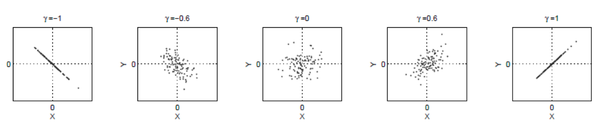
일차원 데이터 $\mathbf {x} \sim \mathcal {N} (0, 1)$와 노이즈(Noise) $\epsilon \sim \mathcal {N} (0, 1)$가 주어질 때, $y = \gamma \mathbf {x} + \sqrt {1 - \gamma^2} \epsilon$ 신호가 출력된다고 하자. 이때, 신호 대 잡음비는 $\frac {\gamma^2}{1 - \gamma^2}$다.

SNR(Signal-to-Noise-Ratio):
$$SNR = \frac {P_{signal}}{P_{noise}} = \left (\frac {A_{signal}}{A_{noise}} \right )^2$$

이제, 일차원 데이터 $\mathbf {x} \in \mathbb {R}$가 주어졌을 때, 클래스 $\circ$에서 $N_{\circ}$개의 데이터를, 클래스 $\triangle$에서 $N_{\triangle}$개의 데이터를 관찰한다고 하자. 이때, $\mathbf {x}_{\circ}$와 $\mathbf {x}_{\triangle}$의 분류를 위한 신호 대 잡음비는

$$\frac {(\frac {1} {N_{\circ}} \sum^{N_{\circ}}_{n = 1} \mathbf {x}_{\circ}) - (\frac {1} {N_{\triangle}} \sum^{N_{\triangle}}_{n = 1} \mathbf {x}_{\triangle})} {\sqrt {(\frac {1} {N_{\circ}} \sum^{N_{\circ}}_{n = 1} \mathbf {x}_{\circ}^2) + (\frac {1} {N_{\triangle}} \sum^{N_{\triangle}}_{n = 1} \mathbf {x}_{\triangle}^2)}}$$

이며, 이를 통계학에서는 t-값(t-value)이라고 부른다.

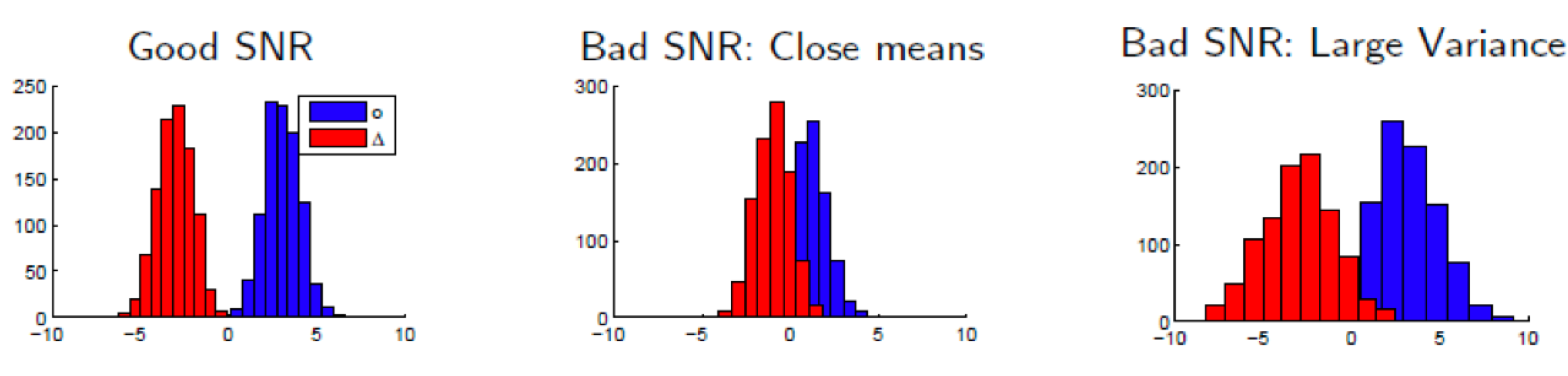
피셔의 LDA는 두 클래스의 평균이 가까워 혹은 분산이 너무 커 두 클래스 데이터가 중첩할 때에 해결책이 될 수 있다.

※ [Machine Learning] NCC(Nearest Centroid Classifier) ← SNR이 안 좋을 때 쓰면 나쁜 예

[Machine Learning] NCC(Nearest Centroid Classifier)

---

LDA(Linear Discriminant Analysis)

※ [Machine Learning] 선형 분류(Linear Classifier)

[Machine Learning] 선형 분류(Linear Classification)

---

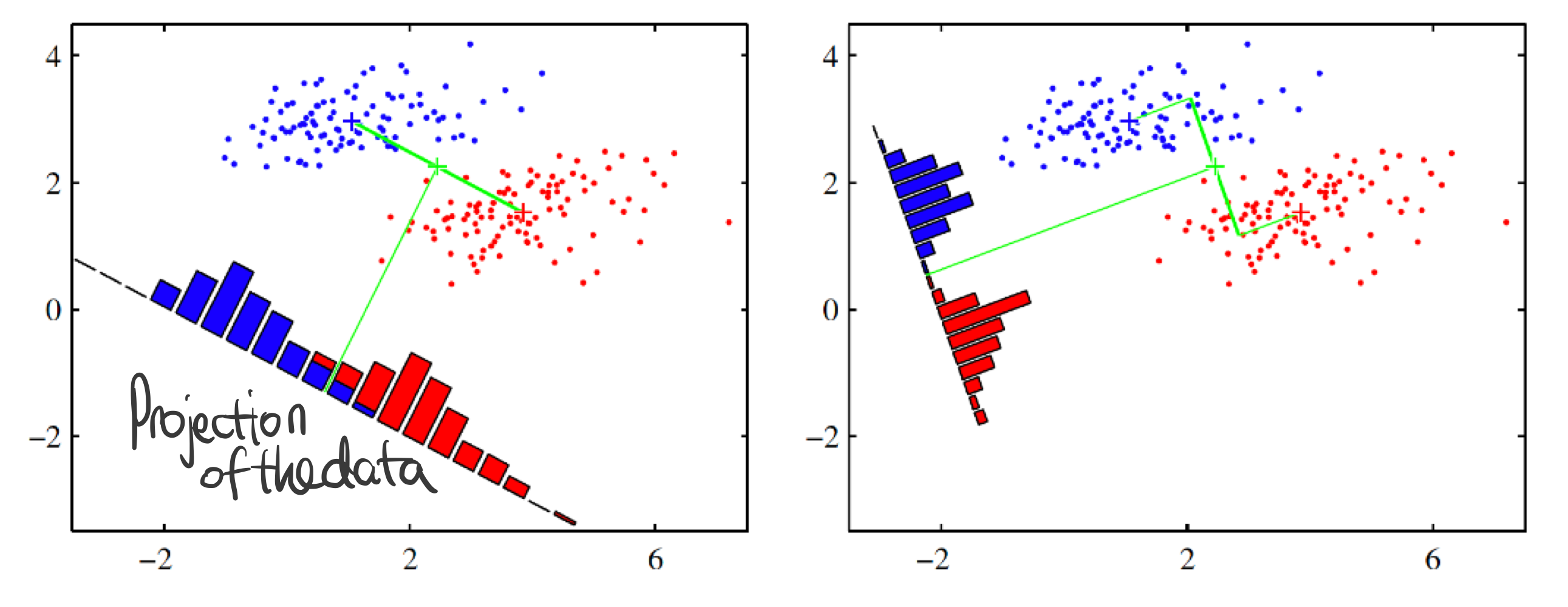
머신러닝을 분류 문제를 차원 축소 문제, 즉, 회귀(Regression) 측면으로 바라보면 다음 그림과 같다.

좋은 선형 분류 모델을 학습하기 위해서는

• 클래스 차이를 최대화하는
  $$(\mathbf {w}^{\top} \mathbf {w}_{\circ} - \mathbf {w}^{\top} \mathbf {w}_{\triangle})^2 = \mathbf {w}^{\top} \underbrace {(\mathbf {w}_{\circ} - \mathbf {w}_{\triangle}) (\mathbf {w}_{\circ} - \mathbf {w}_{\triangle})^{\top}}_{\text {Between Class Scatter } S_B} \mathbf {w}$$
• 그리고 각 클래스의 분산을 최소화하는
  $$
  \begin {split}
  & \frac {1}{N_{\circ}} \sum^{N_{\circ}}_{i = 1} \left ( \mathbf {w}^{\top} (\mathbf {x}_{\circ i} - \mathbf {w}_{\circ}) \right )^2 + \frac {1}{N_{\triangle}} \sum^{N_{\triangle}}_{j = 1} \left ( \mathbf {w}^{\top} (\mathbf {x}_{\triangle j} - \mathbf {w}_{\triangle}) \right )^2 \\
  &= \mathbf {w}^{\top} \underbrace {\left ( \frac {1}{N_{\circ}} \sum^{N_{\circ}}_{i = 1} (\mathbf {x}_{\circ i} - \mathbf {w}_{\circ})(\mathbf {x}_{\circ i} - \mathbf {w}_{\circ})^{\top} + \frac {1}{N_{\triangle}} \sum^{N_{\triangle}}_{i = 1} (\mathbf {x}_{\triangle i} - \mathbf {w}_{\triangle})(\mathbf {x}_{\triangle i} - \mathbf {w}_{\triangle})^{\top} \right )}_{\text {Within Class Scatter } S_W} \mathbf {w}
  \end {split}$$

선형 판별 함수 $\mathbf {w} \in \mathbb {R}^D$를 찾아야 한다.

따라서 피셔의 기준(Fisher Criterion)을 하나의 식으로 표현하면 다음과 같다.

$$arg \max_{\mathbf {w}} \frac {\mathbf {w}^{\top} S_B \mathbf {w}}{\mathbf {w}^{\top} S_W \mathbf {w}}$$

위의 식을 최적화하기 위해 $\frac {\partial}{\partial \mathbf {w}} \left ( \frac {\mathbf {w}^{\top} S_B \mathbf {w}}{\mathbf {w}^{\top} S_W \mathbf {w}} \right ) = 0$을 푼다.

$$
\begin {align*}
\frac {(\mathbf {w}^{\top} S_W \mathbf {w}) S_B \mathbf {w} - (\mathbf {w}^{\top} S_B \mathbf {w}) S_W \mathbf {w}}{(\mathbf {w}^{\top} S_W \mathbf {w})^2} &= 0 \\
(\mathbf {w}^{\top} S_B \mathbf {w}) S_W \mathbf {w} &= (\mathbf {w}^{\top} S_W \mathbf {w}) S_B \mathbf {w} \\
S_W \mathbf {w} &= S_B \mathbf {w} \underbrace {\frac {\mathbf {w}^{\top} S_W \mathbf {w}}{\mathbf {w}^{\top} S_B \mathbf {w}}}_{\text {scalar}}
\end {align*}
$$

$$\therefore arg \max_{\mathbf {w}} \frac {\mathbf {w}^{\top} S_B \mathbf {w}}{\mathbf {w}^{\top} S_W \mathbf {w}} \rightarrow S_W \mathbf {w} = S_B \mathbf {w} \lambda$$

클래스 간 분산(Between Class Scatter) 중 뒷부분이 스칼라이므로 $S_B \mathbf {w} = (\mathbf {w}_{\circ} - \mathbf {w}_{\triangle}) \underbrace {(\mathbf {w}_{\circ} - \mathbf {w}_{\triangle})^{\top} \mathbf {w}}_{\text {scalar}}$, 결론적으로 최적의 $\mathbf {w}$는 다음과 같이 비례하다.

$$\mathbf {w} \propto S^{-1}_{W} (\mathbf {w}_{\circ} - \mathbf {w}_{\triangle})$$

---

예 1) 제한 조건 $\mathbf {w}^{\top} S_W \mathbf {w} = 1$이 있는 LDA 목적 함수

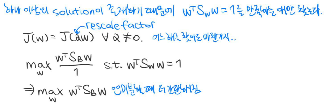
최적화 문제를 라그랑주 승수법(Lagrange Multipliers)으로 풀어 일반적인 고윳값 찾기 문제와 동일한 문제임을 증명했다.

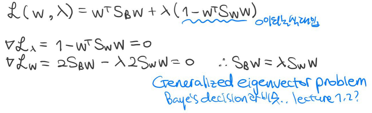
따라서 최적화 문제의 답은 다음과 같다.

---

예 2) LDA의 유계 오차(Bounded Error of LDA)

공분산이 같은 가우시안 분포(Gaussian Distribution)를 가지는 데이터의 사후 확률(Posterior Probability) $P(w | \mathbf {x})$를 최적화 문제와 피셔의 판별식은 같다. 피셔의 LDA의 분류 유계 오차를 살펴봄으로써 평균과 공분산이 오차에 어떻게 영향을 끼치는지 알아보고자 한다.

두 개의 확률 분포로 데이터가 생성된다고 하자. $$P(\mathbf {x} | w_1) = \mathcal {N} (\mu, \Sigma), P(\mathbf {x} | w_2) = \mathcal {N} (-\mu, \Sigma) \text { with } \mathbf {x} \in \mathbb {R}^d$$

베이즈 오류율(Bayes Error Rate):
$$P(error) = \int^\infty_\infty P(error | \mathbf{x})p(\mathbf {x}) d\mathbf{x}$$

다음과 같이 위로 유계(Upper-bounded) 조건부 오차(Conditional Error)를 구할 수 있다.

다음과 같이 위로 유계 베이즈 오류율을 구할 수 있다.

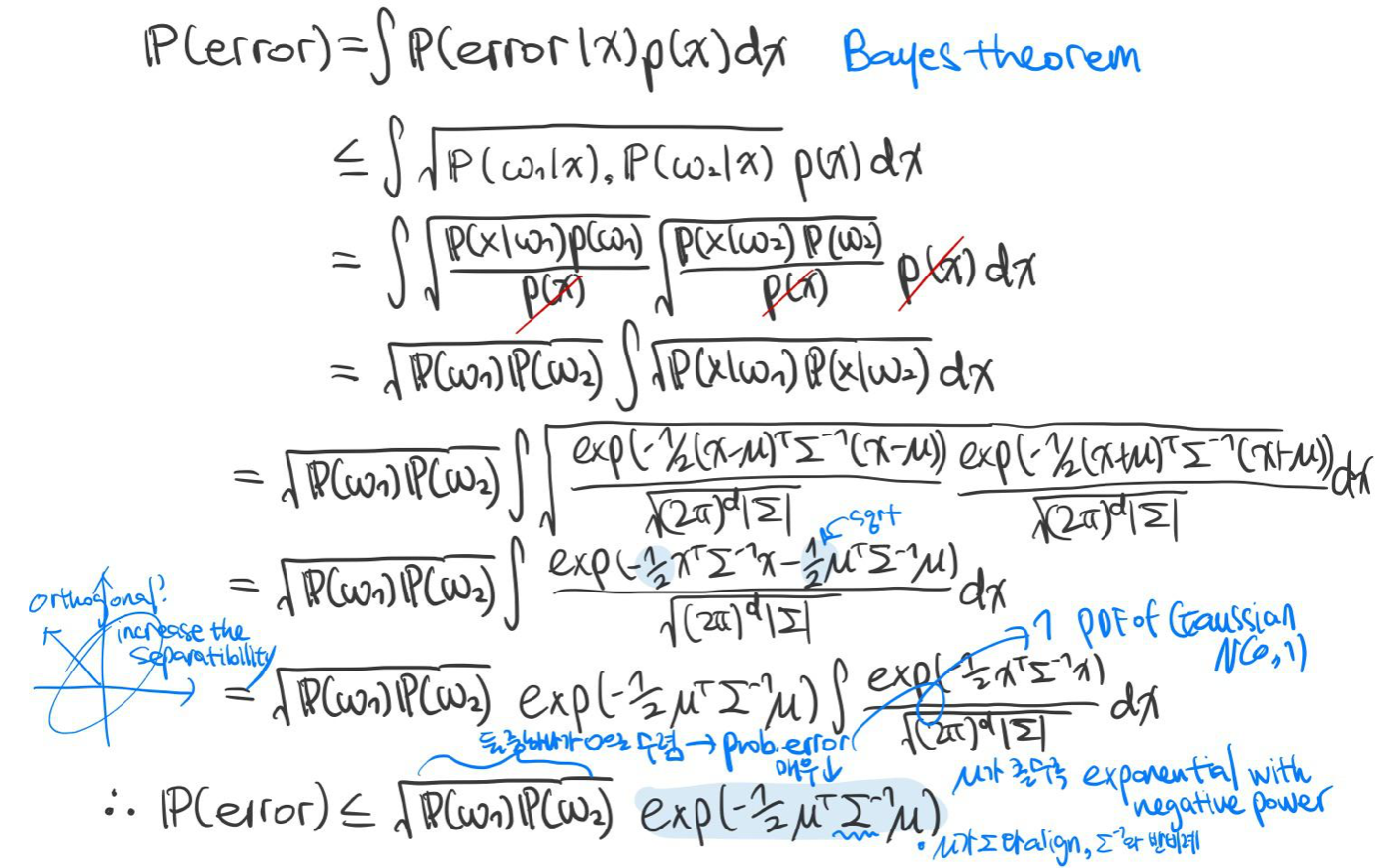
베이즈 결정 이론(Bayes Decision Theory)에서 배웠듯이, 사전 확률(Prior Probability) $P(w)$ 둘 중 하나가 0으로 수렴할 수록 베이즈 오류율은 매우 작아진다. 그 이유는 분류기가 항상 사전 확률이 큰 쪽으로 분류하는 경향을 갖으며, 아주 작은 확률로 사전 확률이 작은 쪽으로 잘못 분류되기 때문이다.

또, 평균 $\mu$가 클 수록 기하급수적으로 베이즈 오류율이 감소한다. 두 클래스의 평균의 차이가 클 수록 SNR은 증가하기 때문에 더 정확하게 분류할 수 있다.

---

LDA와 퍼셉트론의 비교(Comparison of LDA and Perceptron)

[Machine Learning] 퍼셉트론 인공신경망(Perceptron Artificial Neural Network)

---

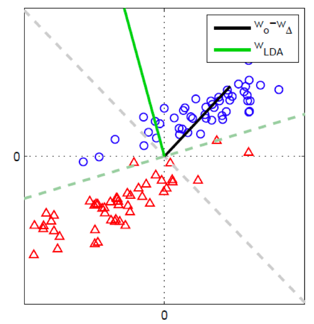
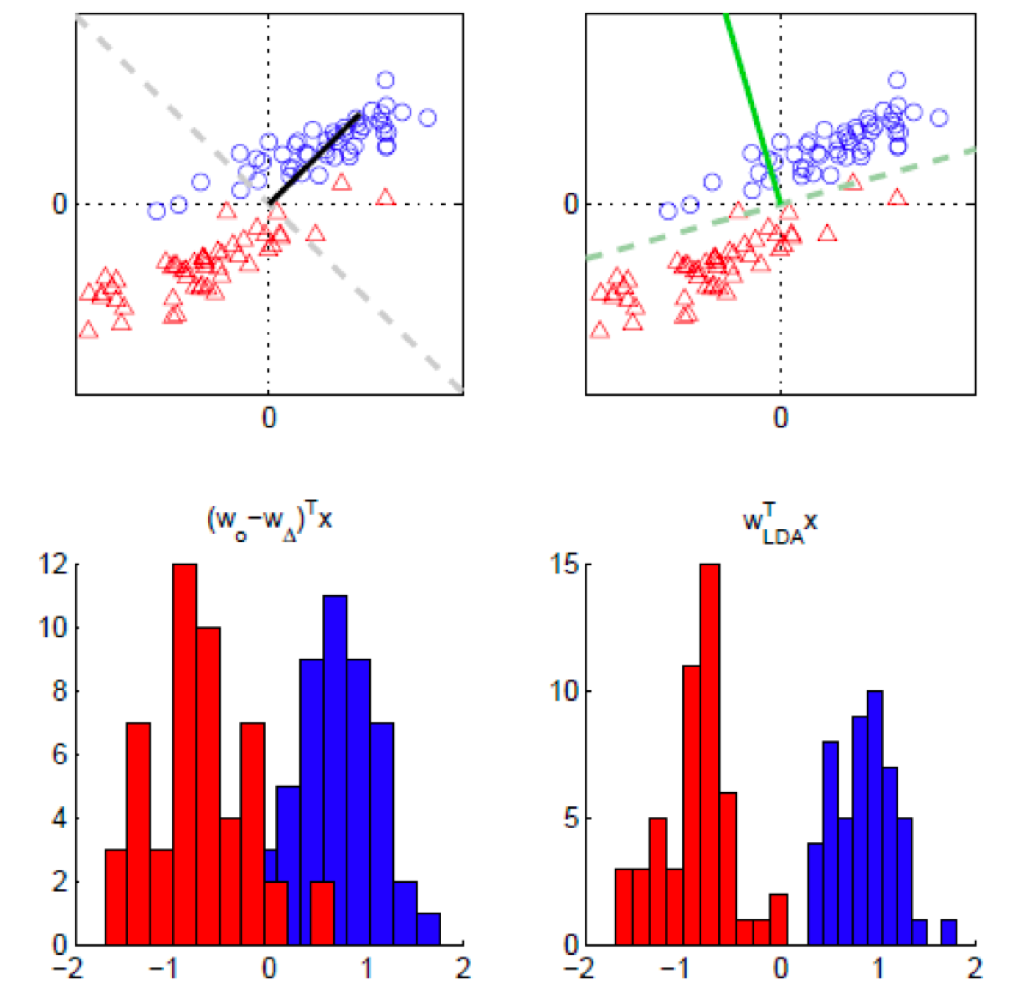
LDA는 클래스 간 분산을 최대화하고 클래스 내의 분산을 최소화한다. 이는 위의 예제에서도 살펴볼 수 있다. 두 클래스의 선형 판별 모델을 데이터 축소의 측면으로 바라보았을 때, LDA가 두 클래스 내의 분산을 최소화한다는 점에서 퍼셉트론의 성능을 뛰어넘었다.

---

[Machine Learning] 공분산 행렬(Covariance Matrix)

만약 두 클래스가 같은 공분산 행렬(Covariance Matrix)을 가질 때, LDA는 먼저 데이터를 비상관화(Decorrelate)한 후 NCC를 적용한다.

$$
\begin {split}
\mathbf {x} \mapsto sign (\mathbf {w}^{\top} \mathbf {x} - \beta)\\
\mathbf {w} \propto S^{-1}_{W} (\mathbf {w}_{\circ} - \mathbf {w}_{\triangle}
\end {split}
$$

$$
\begin {split}
\mathbf {w}^{\top} \mathbf {x} = (\mathbf {w}_{\circ} - \mathbf {w}_{\triangle})^{\top} S^{-1}_{W} \mathbf {x} = \underbrace {(\mathbf {w}_{\circ} - \mathbf {w}_{\triangle})^{\top} \cup \vee^{-\frac {1}{2}}}_{\begin {split} \text {mean class difference} \\ \text {of decorrelated data} \end {split}} \underbrace {\vee^{-\frac {1}{2}} \cup^{\top} \mathbf {x}}_{\text {decorrelated } \mathbf {x}} \\
\text {where } S_{W} = \cup \vee \cup^{\top} \text { is the eigenvalue decomposition of } S_{W}
\end {split}
$$

---

예 1) 피셔 판별식 $\mathbf {w}$

두 개의 클래스 $w_1, w_2$와 각 클래스와 연관된 데이터의 우도(Likelihood)를 다음과 같이 가정하자.

$$p(\mathbf {x} | w_1) = \mathcal {N} \left ( \begin{pmatrix} -1 \\ -1 \end {pmatrix} , \begin{pmatrix} 2 & 0 \\ 0 & 1 \end {pmatrix} \right), p(\mathbf {x} | w_2) = \mathcal {N} \left ( \begin{pmatrix} +1 \\ +1 \end {pmatrix}, \begin{pmatrix} 2 & 0 \\ 0 & 1 \end {pmatrix} \right)$$

피셔의 판별식 $\mathbf {w}$은 다음과 같이 구할 수 있다.

반대로 $arg \min_{\mathbf {w}} \frac {\mathbf {w}^{\top} S_B \mathbf {w}}{\mathbf {w}^{\top} S_W \mathbf {w}}$를 만족하는 $\mathbf {w}$를 계산하면 다음과 같다. 

---

LDA의 한계

LDA의 목적 함수(Objective Function)는 이차 방정식(Quadratic)의 형태를 가지며 이를 계산하기 위해 경험적 평균(Empirical)을 요구한다. 이상치(Outlier)가 존재 시 경험적 평균의 값에 큰 영향을 주기 때문에 효과적으로 LDA를 사용할 수 없다. 

---

1. Richard O. Duda, Peter E. Hart, and David G. Stork. 2000. Pattern Classification (2nd Edition). Wiley-Interscience, USA.

2. Müller, K.R., Montavon, G. (2021). Lecture on Machine Learning 1-X. Technische Universität Berlin, Berlin, Germany.